GStreamer and Gaussianblur: Divide and conquer

One target, two strategies

One of Fluendo's offers is optimizing existing products as part of our Consulting Services. As a team constantly looking for new challenges, we were excited when an electronics and embedded firmware design company trusted us again to sharpen the image their camera was sending without compromising the latency. And we did it using Gaussian blur, a visual effect used in image processing.

Gaussian blur is a well-known element used to primarily blur frames. However, the same algorithm also works to sharpen frames. In this case, our client was required to sharpen the image the camera was sending without compromising the latency. We did research to try to find the most suitable element. The best choice would be to have an encoder support this feature. However, given the target machine, the hardware encoder was not able to perform that task. So, we chose the GStreamer gaussianblur element to do it.

Gaussian blur is a well-known element used primarily to blur frames, but its algorithm also sharpens frames. We researched the most suitable element and thought the best choice would be to have the machine encoder able to support this feature. However, given the target machine, the hardware encoder could not perform that task, so we chose the GStreamer gaussianblur element to do it.

Gaussianblur has an AYUV format for input and output, with raw video data. AYUV is a not-so-common input/output format, so for most cases, a pair of format conversions are needed in the pipeline, as it is in our case. Luckily, liborc helped us do it faster. What’s the problem now? Latency is heavily affected by the software filter. In this blog post, we will explain how we try to deal with that in the following chapters.

GStreamer Latency for gaussianblur

This is the pipeline we used to get the baseline timings:

GST_DEBUG="GST_TRACER:7"
GST_TRACERS="latency(flags=pipeline+element)"
GST_DEBUG_FILE=trace.log
gst-launch-1.0 videotestsrc num-buffers=300 !
"video/x-raw,width=640,height=480" ! videoconvert ! gaussianblur sigma=-2 !
videoconvert ! autovideosink

GStreamer latency statistics

0x557f382a2f10.videotestsrc0.src|0x557f382aa030.autovideosink0.sink:
mean=0:00:00.038152925 min=0:00:00.034853550 max=0:00:00.056464882

Element Latency Statistics:
0x557f382ba1e0.capsfilter0.src:
mean=0:00:00.000022460 min=0:00:00.000013581 max=0:00:00.000046450
0x557f38296210.videoconvert0.src:
mean=0:00:00.000022690 min=0:00:00.000011367 max=0:00:00.000058856
0x557f382a70d0.gaussianblur0.src:
mean=0:00:00.037845591 min=0:00:00.034616857 max=0:00:00.056102031
0x557f382a7780.videoconvert1.src:
mean=0:00:00.000262258 min=0:00:00.000144097 max=0:00:00.000954067

The above data means that our baseline time per frame is around 38ms. All the tests presented here were done in an Intel 11th Gen Intel(R) Core(TM) i7-1165G7 @ 2.80GHz.

Strategy 1. Reduce the number of operations

The gaussianblur filter blurs or sharpens the image based on its own generated kernel. That kernel size depends on the sigma value provided. The lower the value, the sharper the image; the higher the value, the blurred the image.

The kernel size is given by the following formula based on sigma:

center(sigma) = ceil (2.5 * abs (sigma))
kernelsize(center) = 1 + 2 * center

The sigma range goes from [-20, 20], so we can generate kernel sizes from [1, 101]. In our case, we were working with sigma=-2 and had a kernel size of 11 elements. Of course, applying a kernel size of 11 elements by software to each frame has a significant cost, so we tried to work on that for this strategy.

The idea is to use a kernel with a lower size that generates a similar effect by applying the same algorithm. So, we tried to understand the values generated with sigma=-2:

k = [-0.008812, -0.027144, -0.065114, -0.121649, -0.176998, 1.799435, -0.176998, -0.121649, -0.065114, -0.027144, -0.008812]

The function that generates the kernel values what it does is to wrap the center value (1,799435) by values that compensate the sum up to 1, i.e., the remaining values compensate the center. The sum up of the array is equal to one. The farther the value is to the center, the lower its weight, making it less important.

The latency we were experiencing with the filter was very high with a sigma=-2. With the previous premise, we generated a kernel of size 3 with custom values that try to render a similar effect. The values we manually tweaked were:

k = [-0.319168, 1.638336, -0.319168]

Those values generate frames good enough for the client, while the latency is heavily reduced compared to the auto-build kernel. In the proposed GStreamer MR we include a new property to decouple the kernel size and values from the algorithm. So, it is possible to build a kernel based on the sigma value as usual and provide your own kernel as well.

Strategy 2. Split operations across CPUs

We also realized another feature of the algorithm: it used only one CPU to perform all this work. Can this be parallelizable? It mostly walks through the rows of the frame to apply the kernel values. Indeed, it does not work exactly row by row, but it firstly processes [0, center] rows without compensating the values, then processes and compensates all the values (this is the parallelizable part), and finally compensates the [height-center, height] rows.

So, we have a bunch of rows, exactly height – center*2, to be parallelized. We don’t expect a linear speed-up, but it seems that much work can be split.

To do that, we follow this methodology:

• First, create a test for the gaussianblur element to ensure the filter still works properly.
• Second, we did a refactor in the algorithm because some dependencies needed to be cleaned to be parallelized.
• Third, we chose OpenMP to let divide the rows' work into different threads.

Benchmarking

Strategy 1

Image similarities

We are going to generate the sharpness values from the variance of the Laplacian of the image for each case:

	Original	sigma=-2	Independent kernel
Variance (Laplacian)	8211.10	17440.53	16820.10

OpenCV Python code to calculate the sharpness:

laplacian = cv2.Laplacian(image, cv2.CV_64F)
variance = laplacian.var()

Visual results

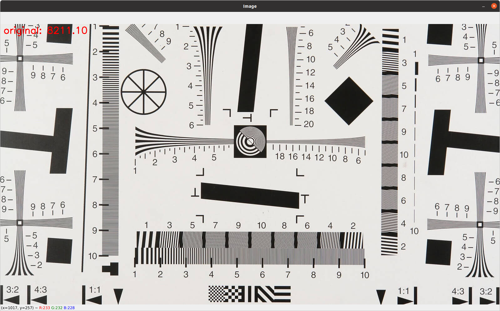
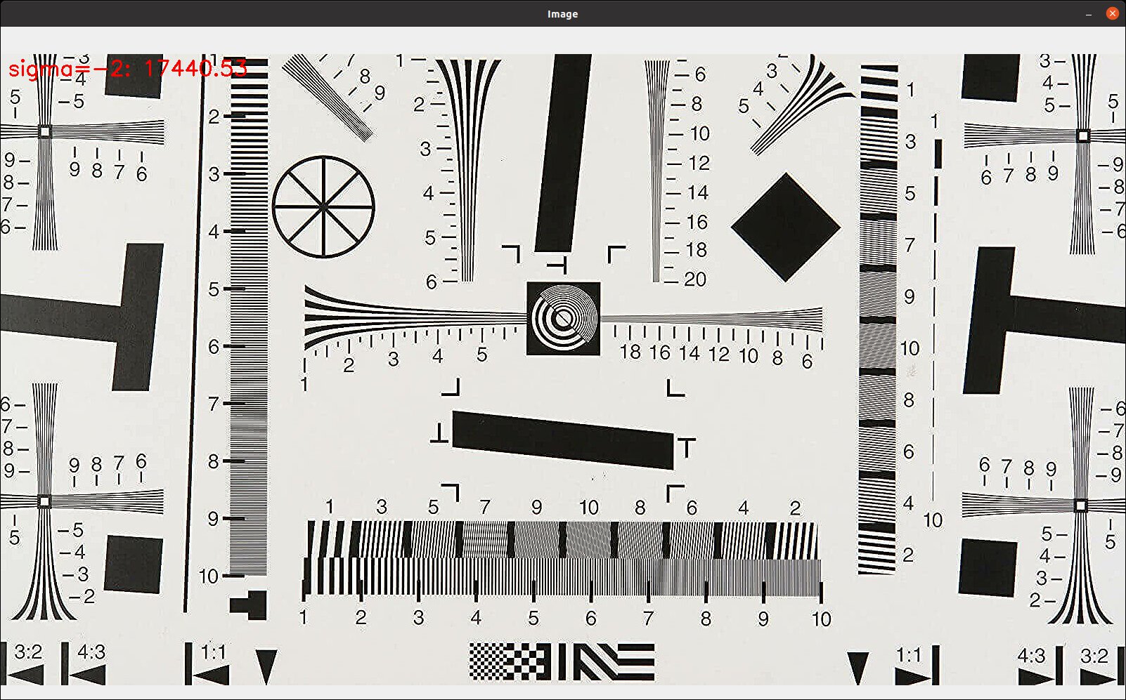
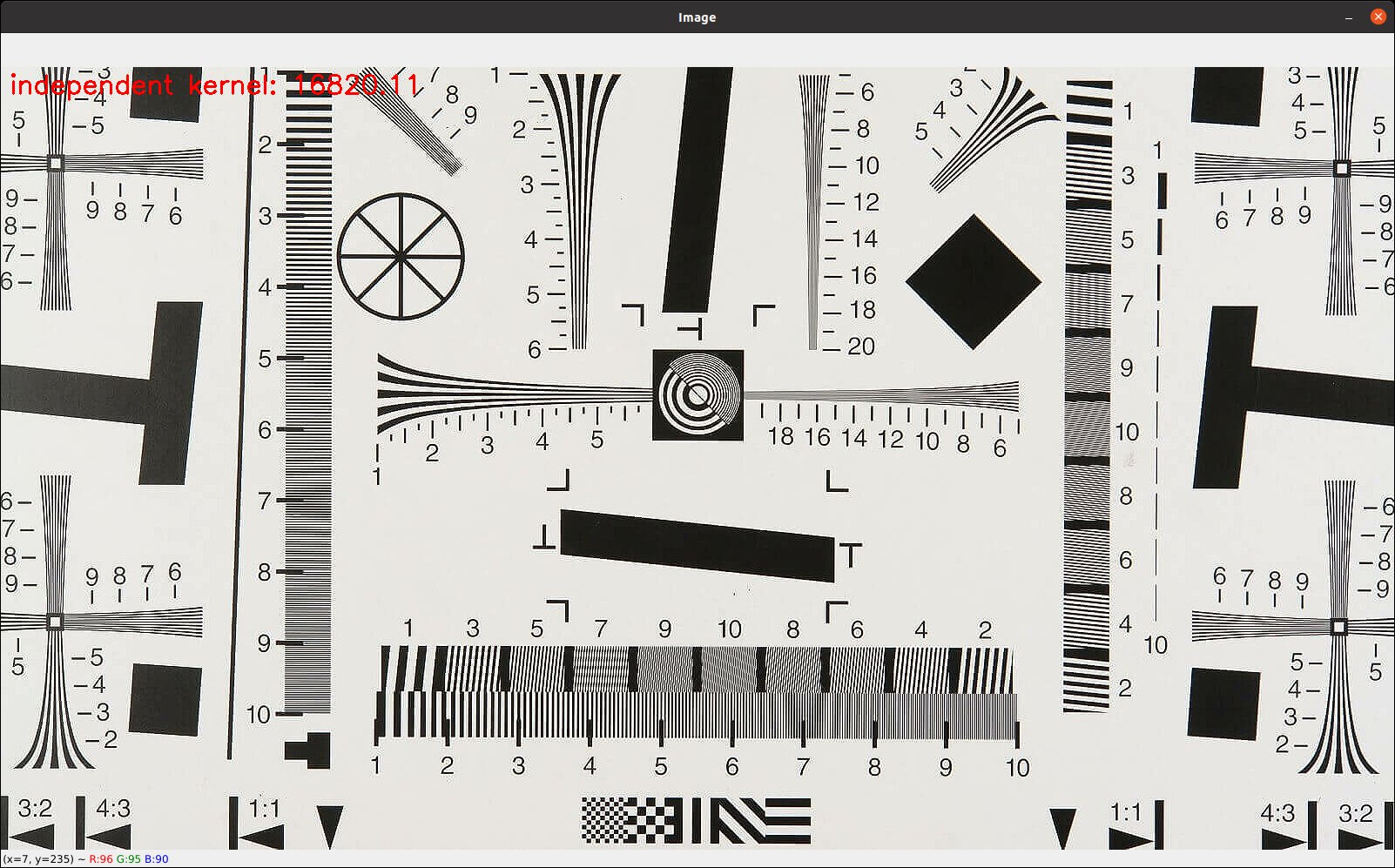
From the values obtained, we can extract that applying a reduced kernel with the right-tuned values can achieve results similar to those of a bigger kernel.

GStreamer Latency statistics

Benchmark pipeline

GST_DEBUG="GST_TRACER:7"
GST_TRACERS="latency(flags=pipeline+element)"
GST_DEBUG_FILE=trace.log
gst-launch-1.0 videotestsrc num-buffers=300 !
"video/x-raw,width=640,height=480" ! videoconvert ! gaussianblur kernel-size=3
kernel="<(float)-0.319168, (float)1.638336, (float)-0.319168>" !
videoconvert ! autovideosink

Latency statistics

0x55ee5d424f90.videotestsrc0.src|0x55ee5d440030.autovideosink0.sink:
mean=0:00:00.023077275 min=0:00:00.019473386 max=0:00:00.036093969

Element Latency Statistics:

0x55ee5d4502c0.capsfilter0.src: 
mean=0:00:00.000052009 min=0:00:00.000029312 max=0:00:00.000116847

0x55ee5d43a8d0.videoconvert0.src: 
mean=0:00:00.000066963 min=0:00:00.000028582 max=0:00:00.000418522

0x55ee5d43d4f0.gaussianblur0.src:
mean=0:00:00.022615997 min=0:00:00.019120287 max=0:00:00.035147830

0x55ee5d43dcf0.videoconvert1.src:
mean=0:00:00.000342305 min=0:00:00.000258617 max=0:00:00.001106929

So we reduced from 38ms to 22ms

Strategy 2

Benchmark pipeline

OMP_NUM_THREADS=8
GST_DEBUG="GST_TRACER:7"
GST_TRACERS="latency(flags=pipeline+element)"
GST_DEBUG_FILE=trace.log
gst-launch-1.0 videotestsrc num-buffers=300 !
"video/x-raw,width=640,height=480" ! videoconvert ! gaussianblur sigma=-2 !
videoconvert ! autovideosink

Latency statistics

0x55a6aa17fe40.videotestsrc0.src|0x55a6aa19b040.autovideosink0.sink:
mean=0:00:00.012469981 min=0:00:00.010468940 max=0:00:00.046589339

Element Latency Statistics:

0x55a6aa1ac320.capsfilter0.src:
mean=0:00:00.000033133 min=0:00:00.000021312 max=0:00:00.000147418

0x55a6aa190c10.videoconvert0.src:
mean=0:00:00.000045183 min=0:00:00.000022788 max=0:00:00.000243142

0x55a6aa1978d0.gaussianblur0.src:
mean=0:00:00.012083058 min=0:00:00.010186229 max=0:00:00.045321935

0x55a6aa197f90.videoconvert1.src:
mean=0:00:00.000308605 min=0:00:00.000170210 max=0:00:00.002932739

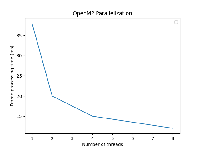
Depending on the height of the frame and the number of threads we get a different speed-up, but in any case, the improvement is clear.

Altogether

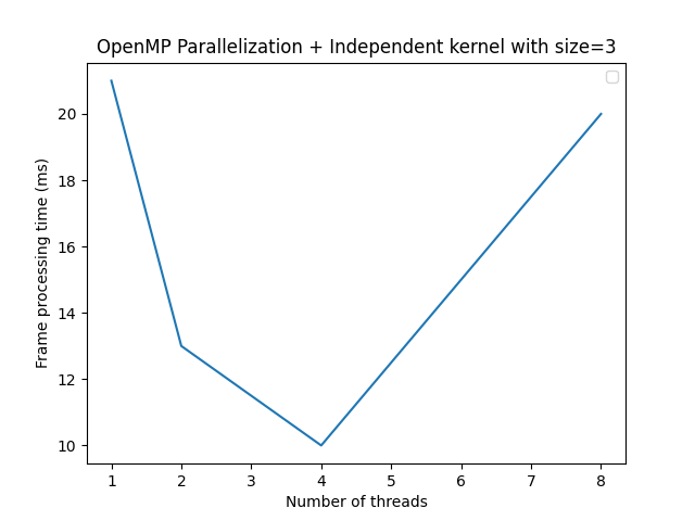
It was interesting to check that by combining both improvements, depending on the number of threads chosen, the performance might not be reached with the maximum number of CPUs. That can be due to when we split the work across CPUs. If the kernel size and data to break are small enough, we waste more time moving data than computing it. So, it’s worth checking each case to see the best choice.

Future work

We did achieve a good improvement in this work; we always want more. Some inner loops in the algorithm can be treated. We parallelized the algorithm in threads to be assigned to different CPUs, but what about using the SIMD features in each CPU as well?

Do you have any multimedia projects in progress? We are your ideal partner for any of them. Whether for training, developing, bug fixing, decoding, encoding, etc. We will be delighted to assist you in achieving your goals. Let’s talk!